Notice
Recent Posts
Recent Comments
NeuroWhAI의 잡블로그
[TensorFlow] MNIST 수행 결과 matplotlib로 이미지와 함께 출력 본문
저는 파이썬 알못이라 matplotlib를 처음 듣지만 파이썬을 주 언어로 사용하시던 분들은 아마 잘 아실듯... 부럽다.
아무튼 이걸로 데이터를 시각화할 수 있다고 합니다.
여기선 MNIST에 있는 손글씨 숫자 이미지를 화면에 뿌려볼겁니다.
1
2
3
4
5
6
7
8
9
10
11
12
13
14
15
16
17
18
19
20
21
22
23
24
25
26
27
28
29
30
31
32
33
34
35
36
37
38
39
40
41
42
43
44
45
46
47
48
49
50
51
52
53
54
55
56
57
58
59
60
61
62
63
64
65
66
67
68
69
70
71
72
73
74
75
76
77
78
79
80
81
82
83
|
import tensorflow as tf
import numpy as np
import matplotlib.pyplot as plt
from tensorflow.examples.tutorials.mnist import input_data
mnist = input_data.read_data_sets("./mnist/data/", one_hot=True)
X = tf.placeholder(tf.float32, [None, 784])
Y = tf.placeholder(tf.float32, [None, 10])
keep_prob = tf.placeholder(tf.float32)
W1 = tf.Variable(tf.random_normal([784, 256], stddev=0.01))
b1 = tf.Variable(tf.random_normal([256], stddev=0.01))
L1 = tf.add(tf.matmul(X, W1), b1)
L1 = tf.nn.relu(L1)
L1 = tf.nn.dropout(L1, keep_prob)
W2 = tf.Variable(tf.random_normal([256, 256], stddev=0.01))
b2 = tf.Variable(tf.random_normal([256], stddev=0.01))
L2 = tf.add(tf.matmul(L1, W2), b2)
L2 = tf.nn.relu(L2)
L2 = tf.nn.dropout(L2, keep_prob)
W3 = tf.Variable(tf.random_normal([256, 10], stddev=0.01))
b3 = tf.Variable(tf.random_normal([10], stddev=0.01))
model = tf.add(tf.matmul(L2, W3), b3)
cost = tf.reduce_mean(tf.nn.softmax_cross_entropy_with_logits(
labels=Y, logits=model
))
optimizer = tf.train.AdamOptimizer(learning_rate=0.001).minimize(cost)
with tf.Session() as sess:
sess.run(tf.global_variables_initializer())
batch_size = 100
total_batch = int(mnist.train.num_examples / batch_size)
for epoch in range(15):
total_cost = 0
for i in range(total_batch):
batch_xs, batch_ys = mnist.train.next_batch(batch_size)
_, cost_val = sess.run([optimizer, cost],
feed_dict={X: batch_xs, Y: batch_ys, keep_prob: 0.8})
total_cost += cost_val
print('Epoch:', '%04d' % (epoch + 1),
'Avg. cost =', '{:.3f}'.format(total_cost / total_batch))
print('완료!')
is_correct = tf.equal(tf.argmax(model, 1), tf.argmax(Y, 1))
accuracy = tf.reduce_mean(tf.cast(is_correct, tf.float32))
print('정확도: %.2f' % sess.run(accuracy * 100,
feed_dict={X: mnist.test.images, Y: mnist.test.labels, keep_prob: 1}))
labels = sess.run(model,
feed_dict={X: mnist.test.images, Y: mnist.test.labels, keep_prob: 1})
fig = plt.figure()
for i in range(10):
# 2x5 그리드에 i+1번째 subplot을 추가하고 얻어옴
subplot = fig.add_subplot(2, 5, i + 1)
# x, y 축의 지점 표시를 안함
subplot.set_xticks([])
subplot.set_yticks([])
# subplot의 제목을 i번째 결과에 해당하는 숫자로 설정
subplot.set_title('%d' % np.argmax(labels[i]))
# 입력으로 사용한 i번째 테스트 이미지를 28x28로 재배열하고
# 이 2차원 배열을 그레이스케일 이미지로 출력
subplot.imshow(mnist.test.images[i].reshape((28, 28)),
cmap=plt.cm.gray_r)
plt.show()
|
cs |
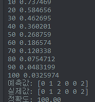
요렇게 실행하고 학습이 끝날때까지 기다리면
Epoch: 0001 Avg. cost = 0.429
Epoch: 0002 Avg. cost = 0.162
Epoch: 0003 Avg. cost = 0.114
Epoch: 0004 Avg. cost = 0.087
Epoch: 0005 Avg. cost = 0.071
Epoch: 0006 Avg. cost = 0.062
Epoch: 0007 Avg. cost = 0.054
Epoch: 0008 Avg. cost = 0.048
Epoch: 0009 Avg. cost = 0.041
Epoch: 0010 Avg. cost = 0.036
Epoch: 0011 Avg. cost = 0.031
Epoch: 0012 Avg. cost = 0.033
Epoch: 0013 Avg. cost = 0.028
Epoch: 0014 Avg. cost = 0.028
Epoch: 0015 Avg. cost = 0.025
완료!
정확도: 97.88
이렇게 나온 다음 아래 창이 뜹니다.

와우!
콘솔창으로 결과를 확인하는것보다 훨씬 이쁘네요.
참고
'개발 및 공부 > 라이브러리&프레임워크' 카테고리의 다른 글
| [TensorFlow] MNIST CNN 예제 고수준 API로 바꾸기 (0) | 2018.01.21 |
|---|---|
| [TensorFlow] MNIST CNN(합성곱 신경망)으로 학습하기 (1) | 2018.01.20 |
| [TensorFlow] 텐서보드 적용 (7) | 2018.01.17 |
| [TensorFlow] 간단한 분류 모델 - 심층 신경망 (0) | 2018.01.10 |
| [TensorFlow] 간단한 분류 모델 (0) | 2018.01.09 |
Comments
'개발 및 공부/라이브러리&프레임워크' Related Articles
more